
A little backstory
So for those of you who don’t know, I have been working as a Backend and AI engineer at Superdash for two weeks at the time I am writing this. And so far, I have worked on voice based AI agents and made them sound more natural. And, I’m sharing whatever I have scratched my head for. You can use this as a extra reading material while building anything related to voice based communication over the internet.
Let’s start with the transfers
Before we dig in the details, let’s see what are some ways to efficiently get your voice or text data from any external API, because unless you are running your own servers, you must be using some TTS provider to get you that sweet sweet voice. Now most commonly, you must have seen either of these ways to get the voice data you want.
- REST API
- WebSockets Streaming
- gRPC
For the average Joe, it is either REST or WebSockets. To build a real time voice agents, you should already be using WebSockets. REST API should only be used if you want to save the voice data to a file, cause it has higher latency and your users wouldn’t like that. So websockets it is, cause it offers low latency, real time streaming and what not. If you are gRPC, you already know more than me what are you dealing with.
So now we have to optimize our websockets to be as fast as it can be, while maintaining a balanced tradeoff with quality. Basically, the only thing affecting the performance is the bandwidth. How much data are we sending over the websockets makes a huge difference in the quality. Send more than what the users need, and you are wasting that precious bandwidth, send less, and the users cannot hear a single word. This is where we step into the world of compression and encoding of audio data.
The glorious land of formats and encodings
When you hear the word audio format, you might think of .mp3, .wav etc etc. But here is a important distinction. These are file extensions, and they represent how the data is packaged or structured. They provide standardized ways for your audio players to read the data and play it as intended. When dealing with AI agents, we mainly use PCM or u-law. So that is what I’ll be covering here.
Why we do not use mp3 for streaming TTS?
In an .mp3 file, the data is stored in sequence of frames, each frame has a compressed data with its relevant header that describes how to decode that frame. Here is a rough visualization of the mp3 file.
+----------------------------+
| Optional ID3 Metadata     | ← Info like title, artist
+----------------------------+
| Frame 1                   |
| ├── Header (4 bytes)      |
| └── Compressed Audio Data |
+----------------------------+
| Frame 2                   |
| ├── Header                |
| └── Audio Data            |
+----------------------------+
| ...                       |
+----------------------------+
Because of the way data is in individual frames, and not continuous, it is not suitable to send in streams, since a partial frame is no good, we need extra frames in the buffer to decode ahead of time, which only introduces more latency. That’s why using mp3 as streaming format will most likely result in choppy audio. This is further complicated by how websockets handle continuous data. MP3 over raw WebSocket or TCP lacks protocol semantics, meaning the websocket has no idea where the data starts or ends, how to deal with packet loss because mp3 frame sizes are variable. The lack of timing information also doesn’t work in the favor mp3, so you need to manually track playback time if you’re synchronizing with other media (like doing any post processing).
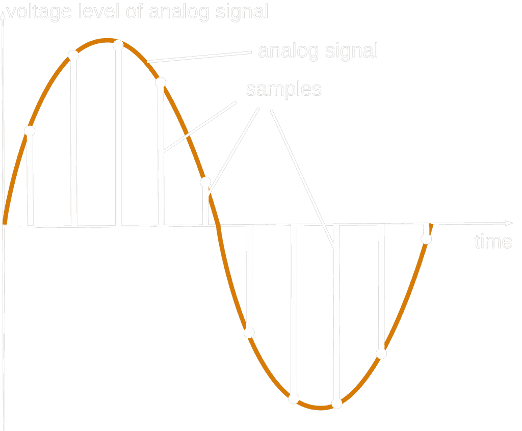
Here comes the PCM
It is the most raw format you can get your audio in. It stands for Pulse-Code Modulation. It represents sound as a sequence of discrete samples, each one capturing the amplitude of the audio waveform at a specific moment in time. And since it is just continuous stream of data, it is very easy to be played while streaming, given the player knows about the properties beforehand, since PCM is headless, it has no metadata to tell the receiver what to expect and how to deal with it.
PCM data if we are saving it in a file container, adds header to it, making it easier to deal with. Typically saved as .wav or .aiff files.
Speaking of properties
While dealing with PCM, you need to agree the following settings:
-
Sample Rate: Defines how many samples taken per second from the analog signal. The bigger the better. Since it is a rate, it is defined in Hz. Typically we use:
- 8,000Hz (8Khz): To use over telephone calls
- 16,000Hz (16Khz): Widely uses TTS standard, speech is crystal clear, helpful if you plan to add some effects or post process the audio further.
- 44,100Hz (44.1Khz): CD Quality, you will rarely need this much data just for speech in AI agents. -
Bit Depth: The number of bits used to represent each sample’s amplitude. Higher bit depth = better dynamic range and less quantization noise.
- 8-bit: Used in μ-law (compressed voice)
- 16-bit: Standard for PCM speech (−32,768 to 32,767)
- 24/32-bit: Music, not used for voice agents -
Byte Order: This defines how the multi-byte values are stored in memory/stream. Basically two main ways:
- Little-endian: Least Significant Bit first (0x01 0x00 = 1) -
Channel Stereo or Mono. Does each of your ear receive its own audio, or the same. For voice agents, we mostly use Mono audio cause we just need voice data. Adding channel only requires more bandwidth..
Putting it all together, Let’s say your ASR model expects:
16 kHz
16-bit signed PCM
Little-endian
Mono
You must send:
[0x3A 0x00][0x2F 0xFF][0x18 0x00]... → Each 2 bytes = 1 sample
If you:
- Send 44.1kHz: Model sees distorted speed/pitch
- Send 8-bit: Model input is too coarse, loses phoneme accuracy
- Send wrong endianness: Sample values are garbage
So far, we are dealing with only linear data. There is another format called μ-law that encodes data in logarithmic scale instead of linear. This provides higher compression ratio making it more suitable for telephony calls since bandwidth there is even more limiting. That’s why telephone providers like Twilio only support sending μ-law audio in 8Khz which is just enough for the other person to hear the voice clearly.
All Hail μ-law
μ-law is a form of non-linear quantization used to encode audio, specifically speech, into a smaller bandwidth while preserving intelligibility. It compresses 16-bit linear PCM into 8-bit samples using a logarithmic scale.
Let’s break down what I just said, say you have a 16-bit signed PCM sample. To convert it into μ-law:
-
Compress it using logarithmic formula:
μ-law(x) = sign(x) * (ln(1 + μ * |x| / Xmax) / ln(1 + μ))where:
μ= 255 (fixed constant)Xmax= max 16-bit PCM value = 32767
-
Quantize to 8 Bits
Quantization is the process of mapping a large set of continuous amplitude values (e.g., 16-bit signed integers) to a smaller set of discrete values (e.g., 8-bit values). It helps in reducing bit depth for compression or transmission, since it is very inefficient to store infinitely precise amplitudes when just sending voice.But why Logarithmic Quantization?
Human speech s not linearly distributed, most meaningful features lie in low amplitudes. μ-law expands quiet amplitudes, making them more discernible even in 8 bits.
The basic maths behind this is just:
F(x) = sign(x) * (ln(1 + μ * |x| / A) / ln(1 + μ))Where:
xis the linear PCM sample (range: −A to +A).Ais the maximum amplitude (usually 32768 for 16-bit PCM).μis a constant (255 for μ-law).sign(x)retains polarity.
This squeezes the linear range into a logarithmic curve, favoring low amplitudes.
-
Adding Bias
Since μ-law uses logarithmic numbers, it becomes undefined where the or problematic for 0 or negative values. The bias ensures:- Avoiding log(0) (which is undefined).
- Shifting the dynamic range to fit the μ-law curve.
- Ensuring better quantization for low amplitude signals (which humans are more sensitive to).
If we skip this step, small signals may get clipped or mapped to the same value and the dynamic range at low amplitudes is lost, which may result in harsh or incorrect audio quality.
2 cents on standards
ITU-T G.711 is the international standard for audio format used in telephony. It defines how to digitally encode analog voice signals using pulse code modulation (PCM) with logarithmic compression (μ-law or A-law).
Adding bias also makes the audio stream complaint to G.711 standard, making it easier to deal when building agents that talk to users over the phone.
What else you can do with this RAW data?
One of things I did to make the voice agent sound more natural and mor life-like is to add some background ambient noise, making it seem that the other person is sitting in some call center in the real world.
On surface, seems like a simple task, just take the voice data, and the background noise data, merge them and send them to the user. Oh, I wish it was as simple as that. So let’s dig a bit deeper into what you can and cannot do with both of these types of formats.
Well if you are just dealing with PCM data, you can actually add the two audio streams, like this:
pub fn mix_audio_p16le(speech_bytes: &[u8], noise_bytes: &[u8]) -> Vec<u8> {
    let len = speech_bytes.len().min(noise_bytes.len());
    let mut mixed = Vec::with_capacity(len);

    for i in (0..len).step_by(2) {
        let speech_sample = i16::from_le_bytes([speech_bytes[i], speech_bytes[i + 1]]);
        let noise_sample = i16::from_le_bytes([noise_bytes[i], noise_bytes[i + 1]]);
        let mixed_sample_i32 = speech_sample as i32 + noise_sample as i32;
        let mixed_sample_i16 = mixed_sample_i32.clamp(i16::MIN as i32, i16::MAX as i32) as i16;
        mixed.extend_from_slice(&mixed_sample_i16.to_le_bytes());
    }
    mixed
}
You should keep one thing in mind, when you add two audio signals, their amplitudes combine. If both your speech and noise are loud, the mixed result can be twice as loud. This can cause the audio to “clip,” which is a gnarly form of distortion you definitely want to avoid.
So what is clipping? In digital audio, every sample has a maximum value it can reach (for 16-bit PCM, it’s 32,767 and -32,768). When you mix two sounds, their sample values are added together. If the new value exceeds the maximum, it gets “clipped” or chopped off. This transforms the nice, smooth sine waves of your audio into harsh-sounding square waves, which sounds like a distorted mess. And once your audio is clipped, that data is gone forever; you can’t get it back.
So, how do we prevent this?
The code snippet above has a slick and simple solution: mixed_sample_i32.clamp(i16::MIN as i32, i16::MAX as i32).
This is a form of hard-limiting. After adding the speech and noise samples, it checks if the result is outside the valid 16-bit range. If it is, it clamps it to the maximum or minimum value. This is a basic way to prevent the harsh distortion of digital clipping, although a more advanced approach would be to use a “limiter” or “compressor” to smoothly reduce the volume before it hits the ceiling. But for real-time mixing, clamping is a super-efficient way to keep things in check.
The issues in playing with volumes
Now, you might be thinking, “To avoid clipping, I’ll just reduce the volume of my PCM audio by multiplying all the samples by, like, 0.5 and then encode it to µ-law.” Intuitively, that makes sense, but in reality, it’s a terrible idea.
Here’s why: µ-law encoding is logarithmic. It’s specifically designed to compress the dynamic range of a 16-bit signal into 8 bits by giving more precision to quieter sounds—which is where most of the important stuff in speech happens—and less precision to louder sounds.
When you scale down your 16-bit PCM audio, you’re effectively making the entire signal quieter. Then, when you convert this quieted-down signal to µ-law, you’re squashing it into the lower, less precise part of the µ-law curve. This leads to a loss of detail and a lower signal-to-noise ratio.The result? The decoded audio will sound flat, muffled, and generally worse than if you had just encoded the original, full-volume PCM to µ-law.
Resampling and Faking New Samples with Interpolation
Sometimes, you’ll get audio in one sample rate, say 48kHz, but you need it in another, like 8kHz for a phone call. The process of changing the sample rate is called resampling. It involves creating a new set of samples at the desired rate. The challenge is figuring out the value of these new samples when they fall between the original ones.
This is where interpolation comes in. It’s a fancy word for generating new data points between existing, known data points. Think of it like “connecting the dots” on a graph. Our code uses a couple of methods for this.
Linear Interpolation: The Straight Line
The most basic way to interpolate is linear interpolation. It just draws a straight line between two existing sample points and picks the value on that line for the new sample.
Check out the linear_interpolate function:
fn linear_interpolate(samples: &[i16], position: f64) -> f64 {
    let idx = position.floor() as usize; // find the last real sample
    let frac = position - idx as f64;   // how far are we to the next sample?

    if idx >= samples.len() - 1 {
        return samples[samples.len() - 1] as f64; // edge case
    }

    let y1 = samples[idx] as f64;     // value of the last real sample
    let y2 = samples[idx + 1] as f64; // value of the next real sample

    y1 + frac * (y2 - y1) // calc the point on the line
}
While it’s fast, the downside is that real audio waveforms aren’t made of straight lines; they’re smooth curves. So, linear interpolation can introduce some high-frequency artifacts, making the audio sound a bit robotic or less natural.
Cubic Interpolation: Getting Curvy
Okay, so we know linear interpolation connects the dots with straight lines. It’s fast, it’s simple, but it’s not how sound works. Real-world sound waves are smooth, continuous curves. When you use straight lines to guess the points in between, you’re creating sharp corners where the lines meet. In the audio world, sharp corners = high-frequency noise. Our ears are super sensitive to this, and it can make the audio sound “phasey,” harsh, or just plain unnatural.
This is where cubic interpolation really shines. Instead of looking at just two sample points, it takes four points into account—the one before the new point, and two after (or two on each side of the gap you’re filling). By looking at this bigger picture, it doesn’t just draw a line; it calculates a smooth curve that passes through all four points. Think about it like this: if you’re trying to guess the path of a baseball, you’d get a much better prediction by looking at the last few feet of its trajectory, not just the last two inches. Why Is a Curve So Much Better?
- It Mimics Reality: Natural sounds don’t jump from one value to another. They transition smoothly. Cubic interpolation, by creating a curve, does a much better job of estimating what the original, analog waveform looked like before it was sampled. It “bends” the interpolated points around the original samples to create a more natural curve.
- Fewer Audible Artifacts: Those sharp corners from linear interpolation can introduce a type of distortion called aliasing. Cubic interpolation’s smooth curves help to minimize these unwanted high-frequency artifacts. The result is cleaner, smoother audio that’s much closer to the original sound. While no interpolation method is perfect, cubic interpolation significantly reduces the “noise” that can be created during resampling.
- It’s the Sweet Spot: There are even more complex methods out there, like windowed-sinc interpolation, but they are much more demanding on the CPU. For many applications, cubic interpolation, specifically a type called Catmull-Rom spline interpolation, hits the sweet spot between high-quality results and computational efficiency. It gives you a huge leap in quality over linear interpolation without bringing your processor to its knees.
Let’s look at the cubic_interpolate function:
fn cubic_interpolate(samples: &[i16], position: f64) -> f64 {
    let idx = position.floor() as usize;
    let frac = position - idx as f64;

    // Fallback to linear if we're at the edges
    if idx == 0 || idx >= samples.len() - 2 {
        return linear_interpolate(samples, position);
    }

    // The four points for our curve
    let y0 = samples[idx - 1] as f64;
    let y1 = samples[idx] as f64;
    let y2 = samples[idx + 1] as f64;
    let y3 = samples[idx + 2] as f64;

    // some math magic to create the curve
    let a0 = y3 - y2 - y0 + y1;
    let a1 = y0 - y1 - a0;
    let a2 = y2 - y0;
    let a3 = y1;

    // calculate the final value
    a0 * frac * frac * frac + a1 * frac * frac + a2 * frac + a3
}
So, in short, while linear interpolation is like a quick “connect-the-dots” sketch, cubic interpolation is more like a skilled artist creating a smooth, flowing line that more accurately represents the original picture. When it comes to audio, that extra bit of artistry makes all the difference.
The Final Takeaway
At the end of the day, working with raw audio for voice agents is a game of trade-offs, precision, and a little bit of math. It’s about understanding that every byte has a purpose, and how you manipulate those bytes directly impacts what the user hears.
I might have been a lot, or too random, from choosing the right transport protocol like WebSockets to diving deep into the DNA of audio with PCM and µ-law. We’ve seen that what seems like a simple task of mixing two audio streams or changing a sample rate, is full of potential pitfalls. If nothing, here is what you can take away from all this:
- Handle Your Levels: Always be mindful of clipping. A simple
clampgets you most of the way there and saves your users’ ears from harsh distortion. - Respect the Format: µ-law is a powerful tool for compression, but its logarithmic nature means you can’t just scale PCM data down without tanking the quality. Encode at the proper volume.
- Don’t Settle for Jagged Edges: When you need to resample, remember that smooth curves beat straight lines. Using something like cubic interpolation instead of linear is a small change in code that makes a huge difference in sound quality.
Ultimately, it’s the sum of these small, deliberate choices that elevates a voice agent from merely functional to truly believable. Getting the audio right is the foundation for creating a fluid, natural, and engaging user experience. And that, after all, is the goal we’re all aiming for.